Showing posts with label ArcGIS. Show all posts

Monday, December 1, 2008

Attribution ADD for you and me

Howdy Dummies. Are you like me? Do you get so wrapped up in mapping lines on high-res imagery that you fail to judiciously attribute them? You know, that 'oh man, I can just keep mapping this obvious contact until it disappears' feeling. Do you do the same with label points (you do use label points, right?)? Well, you can control your attention deficit by selecting a key option in Editor>Options interface:

Once you select the correct attribution option, you will be interrogated by the program as to what the attribute of the feature you just created is. Yes, you will have to make the call then. You really don't have time for that second, or third, or fourth sweep through the map do you? Do it right the first time. Be particularly judicious about your label points since those are much harder to formulate well after the fact.

I had no idea this option was available until fairly recently. If you knew of it, way to go. You are less of a dummy than I.

Friday, September 26, 2008

Masking the lake for a good stretch

If you make your geologic maps using ArcGIS and work with nicely detailed color imagery, then you already know how useful a stretch is. If not, check this previous posts for dummies:


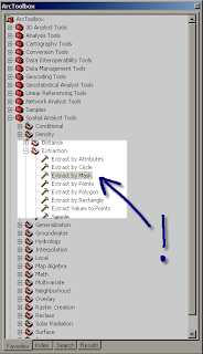
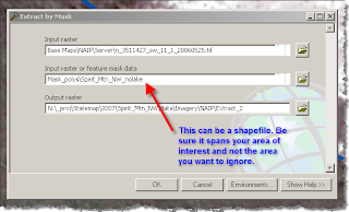
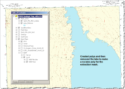
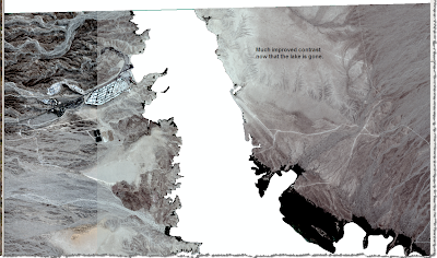
Now that you are back up to speed, I will share a simple trick I figured out by brute force that eliminates areas that may skew your stretch in an inconvenient way. Namely, large bodies of water. Right now, I am supposed to be finalizing mapping in the Spirit Mtn NW quad which includes parts of Nevada, Arizona, and Lake Mohave. Mapping along the lakeshore in the field is a joy; whereas compiling along the lakeshore is a pain in the neck...particularly when you use the standard deviation stretch restricted to the 'current display extent' which is usually the best option for contrast enhancement. The problem is caused by the black hole of lake pixels that dominate the statistics. The solution? Mask out the lake in a new raster using the 'extract' tool:


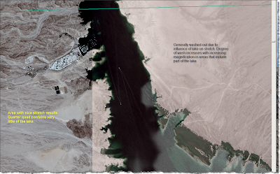
Here are the results from my current map area:

Before:

After:


Epilogue. Someone with considerably more knowledge in GIS than I once explained to me how I could do this with raster math. I screwed around with that and failed. After numerous scans through Arc Toolbox (haven't you scanned that stuff over and over looking for something?), I finally found some commands that sounded useful. Remember, this is digital geoscience for dummies.

Monday, September 22, 2008

How to eat GeoSpaghetti

Geologic mapping can span many scales of time and space. Some of the most complex linework can result from evaluating a fluvial system in great detail in a small area and over a geologically instantaneous period of time. In my case, this scenario corresponds to the Bill Williams River in Arizona. For several years, I have been compiling detailed geologic maps of channel change on that river since 1953. The result? A heaping plate of GeoSpaghetti.
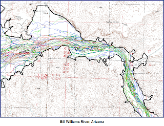
The image above is an excerpt from a 35 mile stretch of river. Yes. The river has undergone some profound changes in the last 50 years or so. Exactly how and why is beyond the point of this blog. One day I will publish it if it matters to you.


The point of this entry is to describe the various tools and methods that I have employed in ArcGIS to compile the lines in a meaningful way and to turn the resulting spaghetti into a meaningful map or series of maps.


The Project:

Map the bottomland geomorphology of the Bill Williams River at specific points in time using a chronology of orthorectified aerial photographs. At this point, I have mapped six generations of the valley bottom. The resulting plexus of lines is a logistical nightmare to a certain extent, but I believe I came up with a reasonable way to deal with them. If you map similar things and have better ideas or suggestions, please let me know.


  1. Set up a geodatabase...yes you need to know the basics of this fundamental operation. Add your lines as classes in a geology feature dataset.
  2. Determine a boundary to which you will be mapping and stick with it. Note that as you map different generations of lines, you will want to alter the boundary...you just will. However, unless it is a major issue and you will diligently propagate that alteration through all of your line layers, resist the temptation
  3. Develop a line and polygon attribution scheme that is flexible and systematic. Important: this scheme needs to be logical and transferable to each generation of linework. Certain generations may require specific types of lines and polygons, but try to adhere to a common conceptual base so that it makes sense all the way through. Record the nomenclature in a spreadsheet and update it when you inevitably revise or add to your units. The spreadsheet can be a life-saver if you tend to work on too many projects and put this one down for a few months.
  4. Begin mapping the earliest generation of photograph if possible. It is best to map the images in chronological order for reasons that will soon become clear. Map lines NOT polygons. Starting with polygons is whacked. You can build them from lines in a matter of seconds.
  5. Once the earliest generation is mapped (and you have attributed the ‘proto’ polygons with a point feature class...post coming if this is news to you) and the topology is all correct (you did build and check the topology, right?) copy it and rename it. Use this dataset as a starting point for the next generation of photos. Note: the tediousness is about to set in or get worse.
  6. Yikes. Your map is already a mess. Now you need to mesh the data in a logical way. You have added lines that preclude the existence of some of the previous generation’s lines, right? All of the precluded lines need to be removed (don't worry the originals still exist...remember, you copied them).
  7. Luckily, you have already built and analyzed the topology of your first layer, right? Well now build and analyze the topology of the second layer for laughs. The only rule you really need is the ‘no dangles’ rule. If you have the topology built and analyzed, you can use the ‘Planarize’ tool to break selected lines (even all of them) at each intersection. Then you can sweep through and select and delete all of the (now) superfluous lines.


That sounds easy right? It is easy, but really really tedious. Also, unless you have taken some preliminary precautions, you may lose all of your careful attribution. For better or worse, when you set up the geodatabase, you have many, many, options to ignore or address. Some of these are very useful to know about. One is ‘Default value’. What you choose here is the default attribution given to any piece of data that you enter. In the case of the Bill Williams map, setting the apyear (aerial photograph year) to the appropriate year was essential and useful. In other cases, I bet you can come up with some examples of your own where this would be useful.


You may also find yourself splitting and merging many lines. Unless you establish 'split' and 'merge' policies, you may get some disconcerting results...like total loss of attribution that you didn't find out about until you split 10s to 100s of lines:


It is best practice to attribute your geolines immediately upon drawing them unless it is really ambiguous and you have a firm follow-up plan. Thus, choosing a default value for a line that requires some scientific judgment may not be the best idea. In the (recent) past, I have had a tendency to map many lines without attribution, assuming that I will do it in a ‘second pass’ through the data. Yikes. That is really stupid. For one thing, once you have drafted the line, you have covered it; for another, the ‘second (or third) pass’ idea isn’t very efficient and just effing snowballs up on you.


So what to do?


Option 1: Diligently attribute each line after you draft it.

Option 2: Have the program force you to attribute the line, or point, or poly, once you draft it.

Option 2 is the most efficient way to go. I just discovered this one.


Stay tuned for updates as to the progress of the Bill Williams River map...polygons coming next.

Thursday, May 29, 2008

Hey Dummy...Quit ignoring GIS Servers in ArcCatalog

Ok. So I am not so smart...big surprise. It is digital geoscience for dummies after all, and I am a geologist, not a GIS-geek. At the DMT meeting last week I was able to have several head-to-heads with some well-trained ESRI representatives. I learned more than I can remember now, but the key thing I learned is the value of the network connection/ gis server function in ArcCatalog. Yes, I have always seen it and always ignored it. Whoops. With recent developments at ArcGIS online, you can link your mxd to various streaming sources of data. If you use ArcGIS, you need to check out ArcGIS online.

I started to get a whiff of this when using Topofusion (see previous posts) and, more recently, Global Mapper, because these programs can load imagery in the background of your project when you are online. Anyway, check this out:


The image above shows my Ivanpah Valley, NV megamap (the flood hazard version) at 1:250k with high resolution ortho imagery in the background. Also, check this out:


ESRI provides a decent data set of shaded relief for the globe. This is what southern Nevada looks like. The shaded relief looks considerably better when zoomed out over a larger region and makes a great overview map.

You can also 'be served' some pretty decent satellite imagery, as shown below:


So, how does this work? Pretty freaking simple. Create Network Connections in ArcCatalog. You just need to decide if it is an ArcGIS server, an ArcIMS server, or an WMS server. Then you simple add the server data source to your active project much as you would imagery or data hosted on your desktop computer. Of potentially great interest is the fact that you can connect to seamless.usgs.gov and choose the data type that you want to add from a long list.


Note: The high resolution imagery available at ArcGIS online is the new color NAIP orthoimagery (I'm pretty sure), so it is completely viable as a geologic mapping supplement. I wish I had known about this long ago. Being self-taught in GIS has its disadvantages. If any of the 4 people out there who may look at this blog know of any other online map services of value to geologists, let me know.

Wednesday, November 28, 2007

Correlation Diagram In Excel--it works(!)

It is possible to develop a decent correlation diagram in Excel. This is an example of a single worksheet incorporated into a workbook with all of the other tabular data supporting a geologic map that I am making of the Owyhee River area, Oregon. Not only is this a good way to keep all of your data in one place (Arc 9.2 can incorporate Excel worksheets quite painlessly now), but this diagram can be directly linked to an mxd file of the map layout. This is a positive development for all concerned parties (the geology team and the cartography team). This sheet is stored amongst sheets that show the point codes, line codes, and unit codes and can be updated concurrently if you stay on top of it.

Note that there are not nearly as many color options in older versions of Excel. The diagram above was created in the newest version.

Thursday, November 8, 2007

Data Points in a Geodatabase

Stations (site specific data)

[kind] O = generic observation

[kind] A = age

[kind] G = graphic data

[kind] R = sample sites

[kind] Y = analytical


Age categories (prefix 1)

a = Argon-Argon

r = radiocarbon

t = tephrochronologic

c = cosmogenic
Graphic data categories

p = photograph

s = sketch
Sample site categories

r = rock


s = sediment

t = tephra

Analytical categories


f = fluvial transport direction

g = fluvial gravel lag

This is the structure of point data that we have built into the geodatabase for the Owyhee River mapping project. It covers all of the ground that is presently relevant to that project, but would need to be modified for a bedrock / structural map, for example.

Monday, October 29, 2007

Geologic Line Standards

OK, this is a long one, but I wanted to illustrate a geodatabase coding scheme for various line types used in geologic mapping with ArcGIS. This rather large subset and the related explanations is drawn from my mapping project on the Owyhee River so it is somewhat specific.

The codes are based on terminology in the new digital geologic map standards published by the FGDC. The underlying scheme is based on one developed by Hastings and Sylvester. The seemingly overly detailed list is based on degrees of certainty relative to two aspects of lines on a geologic map: 1. What sort of line it is and how certain you are about that; and 2. How well the line's location is known.

Each funny looking code is a combination of the following characters that account for a variety of lines and a variety of degrees of certainty about what and where they are:

Line Types [kind]
  • C Contact
  • X Fault
  • R Rock body (marker bed or key bed)
  • Z Scarp (as feature, not contact)
  • M Morphologic
  • B Boundary
Prefixes [category]
  • g generic
  • l landslide
  • i internal
  • f fluvial
  • v volcanic
  • s sedimentary
  • z scarp
  • d depression
  • m morphologic feature
Suffixes [location]
  • c certain
  • q questionable
  • a accurate
  • x approximate
  • c concealed
  • i inferred
Code followed by Name
  • uB Boundary—undifferentiated
  • mB Boundary—mapsheet
  • pB Boundary—property
  • sB Boundary—scratch
  • wB Boundary—water
  • eB Boundary—exclusion
  • gCca Contact—Identity and existence certain, location accurate
  • gCqa Contact—Identity or existence questionable, location accurate
  • gCcx Contact—Identity and existence certain, location approximate
  • gCqx Contact—Identity or existence questionable, location approximate
  • gCci Contact—Identity and existence certain, location inferred
  • gCqi Contact—Identity or existence questionable, location inferred
  • iCca Internal contact—Identity and existence certain, location accurate
  • iCqa Internal contact—Identity or existence questionable, location accurate
  • iCcx Internal contact—Identity and existence certain, location approximate
  • iCqx Internal contact—Identity or existence questionable, location approximate
  • sCca Incised-scarp sedimentary contact—Identity and existence certain, location accurate.
  • sCqa Incised-scarp sedimentary contact—Identity or existence questionable, location accurate.
  • sCcx Incised-scarp sedimentary contact—Identity and existence certain, location approximate.
  • sCqx Incised-scarp sedimentary contact—Identity or existence questionable, location approx.
  • ldCca Sag-pond or closed depression on landslide (mapped to scale)
  • viCca Contact separating individual lava flows within same map unit—Identity and existence certain, location accurate
  • viCcx Contact separating individual lava flows within same map unit—Identity and existence certain, location approximate
  • viCqx Contact separating individual lava flows within same map unit—Identity or existence questionable, location approximate
  • gXca Fault (generic; vertical, subvertical, or high-angle; or unknown or unspecified orientation or sense of slip)—Identity and existence certain, location accurate
  • gXqa Fault (generic; vertical, subvertical, or high-angle; or unknown or unspecified orientation or sense of slip)—Identity or existence questionable, location accurate
  • gXqx Fault (generic; vertical, subvertical, or high-angle; or unknown or unspecified orientation or sense of slip)—Identity or existence questionable, location approximate
  • gXcc Fault (generic; vertical, subvertical, or high-angle; or unknown or unspecified orientation or sense of slip)—Identity and existence certain, location concealed
  • kRca Key bed—Identity and existence certain, location accurate
  • kRcx Key bed—Identity and existence certain, location approximate
  • fZca Fluvial terrace scarp—Identity and existence certain, location accurate. Hachures point down scarp
  • fZqa Fluvial terrace scarp—Identity or existence questionable, location accurate. Hachures point down scarp
  • fZcx Fluvial terrace scarp—Identity and existence certain, location approximate. Hachures point downscarp
  • lZca Head or main scarp of landslide—Active, sharp, distinct, and accurately located. Hachures point down scarp
  • lZcx Head or main scarp of landslide—Inactive, subdued, indistinct, and (or) approximately located. Hachures point down scarp
  • liZca Internal or minor scarp in landslide—Active, sharp,distinct, and accurately located. Hachures point down scarp
  • liZcx Internal or minor scarp in landslide—Inactive, subdued, indistinct, and (or) approximately located. Hachures point down scarp
  • vMca Flow lobe or lava-flow front—Identity and existence certain, location accurate. Hachures on side of overlying younger flow
  • vMqa Flow lobe or lava-flow front—Identity or existence questionable, location accurate. Hachures on side of overlying younger flow
  • vMcx Flow lobe or lava-flow front—Identity and existence certain, location approximate. Hachures on side of overlying younger flow
  • vMqa Flow lobe or lava-flow front—Identity or existence questionable, location approximate. Hachures onside of overlying younger flow
  • vMm Crest line of pressure ridge or tumulus on lava flow

Sunday, October 28, 2007

Mandatory (Basic) Image Enhancements

Smooth Your Image:


To get the most most out of your base imagery, you need to experiment with different image enhancement tools in Arc. The basic manipulations can be found under the 'display' and 'symbology' tabs found under 'layer--properties' (right-click on the layer of interest). To smooth the image without any negative effects, choose the 'bilinear interpolation' option and then click 'apply'. This will smooth your image in a visually satisfying way. Other resampling options may result in bothersome artifacts in the typical types of imagery that geologists use for mapping.

Stretch Your Imagery:

Stretching your image can create levels of contrast and color balance that you will appreciate. For details, consult a remote sensing textbook. For now, just accept the fact that you can vastly improve an image's appearance by applying a standard deviation stretch to your data. Start with n=2 and experiment with increasing and decreasing this value. Also, if you limit the stretch statistics to the 'Current Display Exent' you will get ~local results that typically improve the contrast of the image. This will vary with the absolute range of values present in the current display. Experiment with other stretches.

Both of these enhancements are useful for b/w DOQQs, color DOQQS, and Quickbird data among (presumably) all other remotely sensed base (photo-like) imagery. It is not useful for DRGs.

Geologic Mapping Toolbar in ArcGIS

If you are limited to working with one screen, you will find it useful to make a custom toolbar to assist in compiling a geologic map. Simply right-click on the toolbar area and scroll through the list of available toolbars to the word 'customize', then make and name a new toolbar. You can then drag individual tools (commands) from the long lists of possibilities onto your new toolbar. In some cases, you will find that you have to drag the tool from an existing bar on your screen. The scale tool is an example that comes immediately to mind. The shot above is from my laptop.